3 Prediction
N <- 40
sde <- 89.52
y1 <- b1+b2*x+rnorm(N, mean=0, sd=sde)

y2 <- data.frame()
y2 <- cbind(y1, y)
3.1 Least sqaures prediction (one time)
matplot(y1, type='l', col=1:40,
        xlab='Income', ylab='Food Expenditure',
        main ='Prediction N=1 ')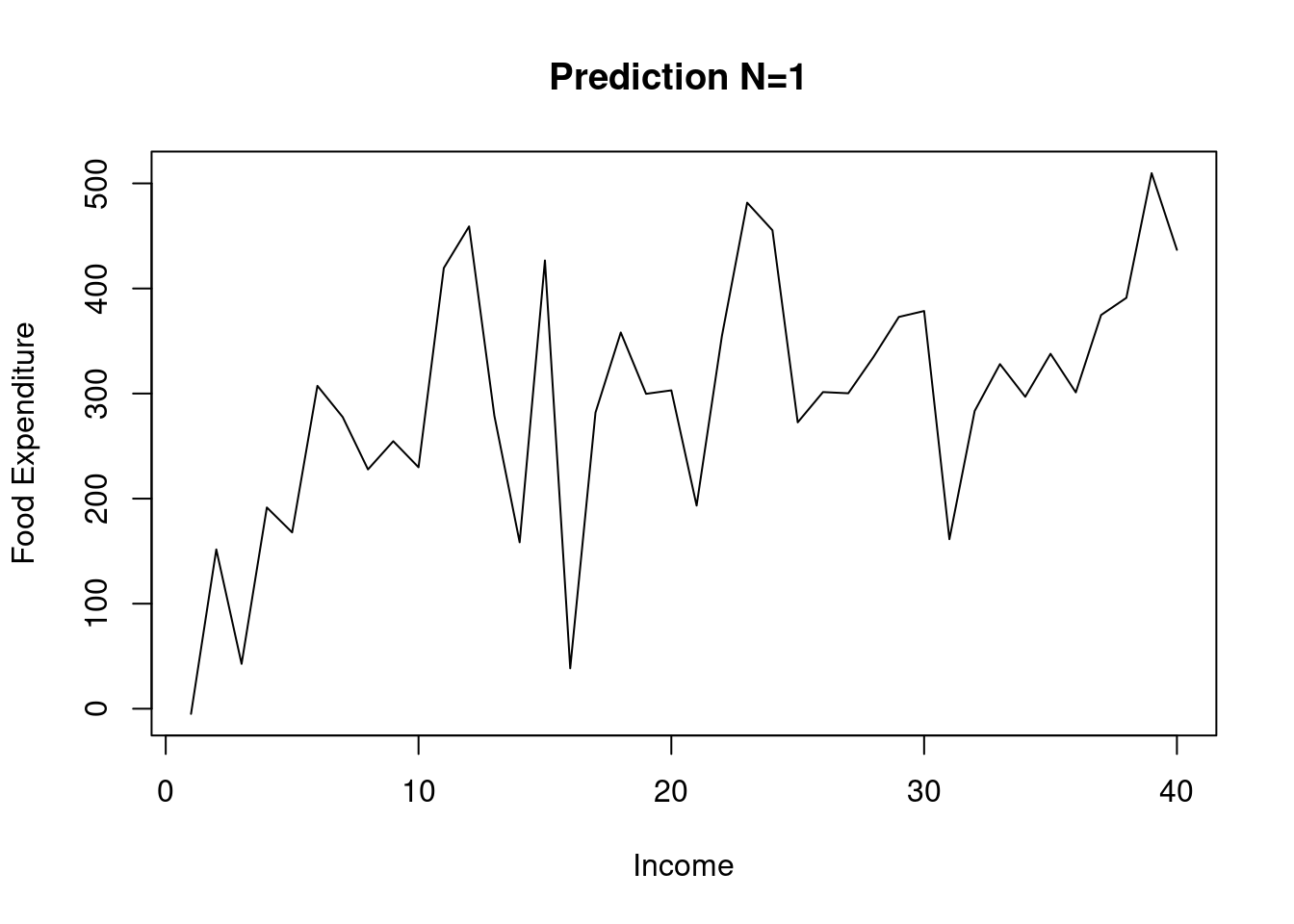
3.2 Least sqaures prediction (one time)
matplot(y2, type='l', col=1:40,
        xlab='Income', ylab='Food Expenditure',
        main ='Food Expenditure vs. Prediction ')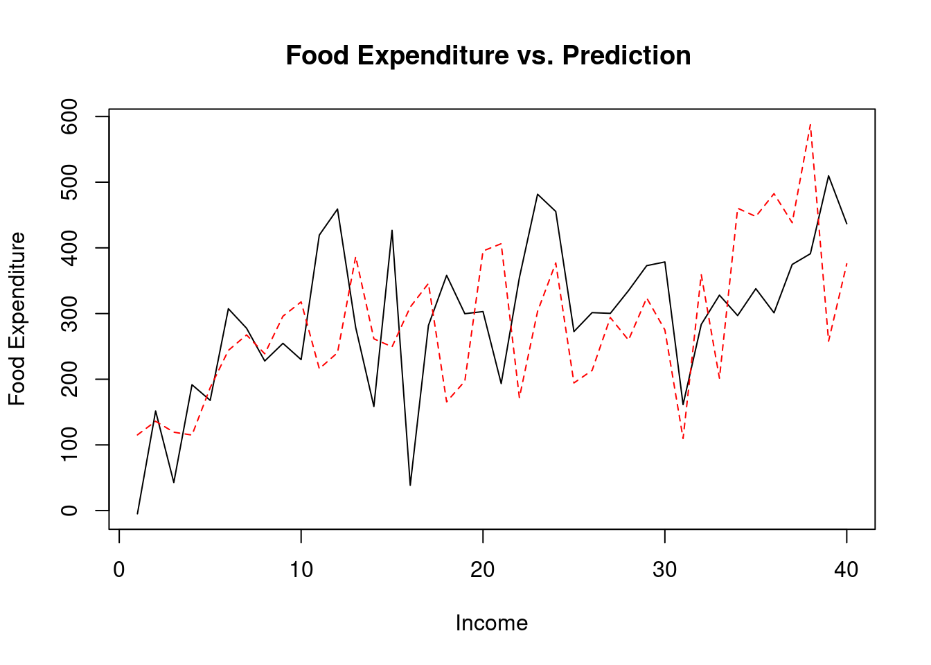
3.3 Least sqaures prediction (1,000 times)
b1 <- coef(reg)[[1]]
b2 <- coef(reg)[[2]]
yy <- data.frame()

trial <- 1
trials <- 1000
while(trial <= trials) {
  y3 <- b1+b2*x+rnorm(N, mean=0, sd=sde)
  yy <- rbind(yy, t(y3))
  trial <- trial + 1
}
3.4 Least sqaures prediction (1,000 times)
matplot(t(yy), type='l', col=1:40,
        xlab='Income', ylab='Food Expenditure',
        main ='Prediction N=1000 ')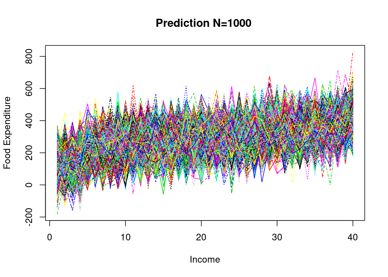
3.5 Save DATA
sink(‘ch4.out’)
# Least sqaures prediction (one time)

y1
## [1] -4.883081 151.632660 42.721901 191.566755 167.833103 307.337831
## [7] 277.627948 227.789231 254.630076 229.824741 419.499320 459.092313
## [13] 278.822266 158.404531 426.675075 38.499510 281.884750 358.132093
## [19] 299.747817 303.030505 193.380462 354.633811 481.665219 455.411110
## [25] 272.588314 301.399430 300.264000 334.927543 372.908323 378.556064
## [31] 161.358288 283.437806 328.006270 296.933456 337.840381 301.100784
## [37] 374.742670 391.104975 509.756569 436.770436sink()